Green Ammonia Facility Financial Model Template

3-Statement Excel Green Ammonia Facility Financial Model Template. A 30-year project finance model built the way a bank would build it — construction through steady-state operations, 31-tab, formula-linked project finance model for a green ammonia facility — from first shovel to final debt maturity.

Financial Model for a Green Ammonia Facilty

This model treats the project the way an infrastructure lender or sponsor actually would: a non-recourse SPV structure with a five-year construction phase, a two-year commissioning ramp, and twenty-four years of steady-state operations, all stitched into one workbook where every number traces back to a handful of core assumptions. Change the PPA price on the Assumptions tab and watch it move through power costs, EBITDA, DSCR, the debt schedule, and equity returns — because that’s what happens in a real financing, and a model that can’t do that isn’t actually a model. Below is what’s on each of the 31 tabs and why it’s built the way it is.

Cover

The front door: what this model is and how it’s built

The Cover tab states plainly what the workbook is — a green ammonia project finance model spanning construction and twenty-four years of operations — and, more importantly, explains the one structural decision that shapes everything downstream: the model runs on an annual backbone for linking revenue, financing, tax, and the three statements together, but drops into full monthly resolution for the construction and commissioning window, where sub-annual timing genuinely changes the answer. It also carries the project name, currency convention, version, and preparation date, along with a full index of the other thirty tabs so anyone opening the file for the first time knows where to go.

Dedicated Downside, Base and Upside sections covers every price scenario

Control

The dashboard: scenario switches and model health at a glance

Control is where the model’s behavior gets toggled rather than edited. A single scenario selector (Base, Upside, or Downside) drives every price, cost, and availability shock elsewhere in the workbook; a cash sweep switch turns optional debt prepayment on or off; a refinancing switch flags whether the Year 10 refinancing scenario is live. Below the switches sits a live readout of the model’s own health — the master check result and error count pulled straight from the Checks tab — so a reviewer can tell in one glance whether the file they’re looking at is internally consistent before they trust a single output.

Summary

The one-page answer: capacity, cost, returns, and whether the model ties out

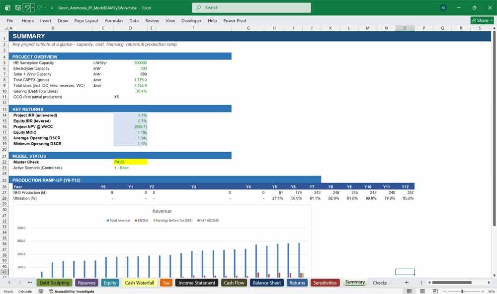
Summary is the page an investment committee actually reads. It pulls together nameplate capacity, total capital cost, gearing, and commercial operations date alongside the headline return metrics — project IRR, equity IRR, NPV, MOIC, and average and minimum operating DSCR — with the active scenario and master check status displayed right next to them. A short production ramp table and two charts, a bar chart of ammonia output climbing from zero through commissioning to full nameplate, and a line chart of the DSCR profile across the debt tenor, turn thirty years of numbers into something you can absorb in ten seconds.

Project IRR
Equity IRR
NPV
MOIC

Assumptions

The single source of truth: every hard-coded input, in one place

Every number a person could reasonably want to change lives on this one tab, organized into clear sections — general and macro, renewable power, electrolyzer, nitrogen and ASU, ammonia synthesis, revenue, opex, capital structure and debt, and tax and incentives — with sixty-seven individually labeled inputs, each carrying its unit and a short note on where it comes from. Nothing downstream is hard-coded a second time; every other tab in the workbook reaches back to a specific cell here, which means recalibrating the model for a real project, a different site, a different offtake structure, is a matter of editing this one tab, not hunting through thirty others.

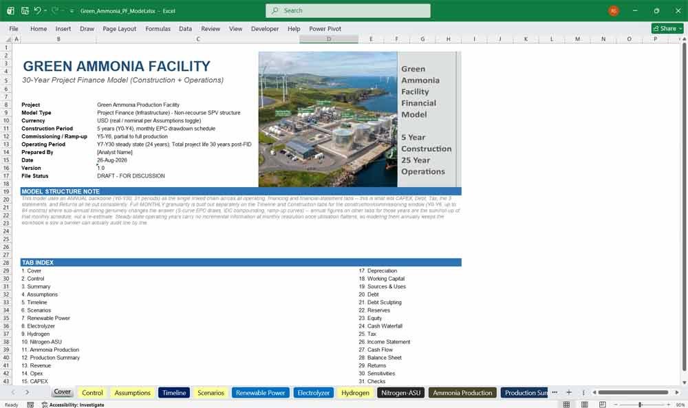
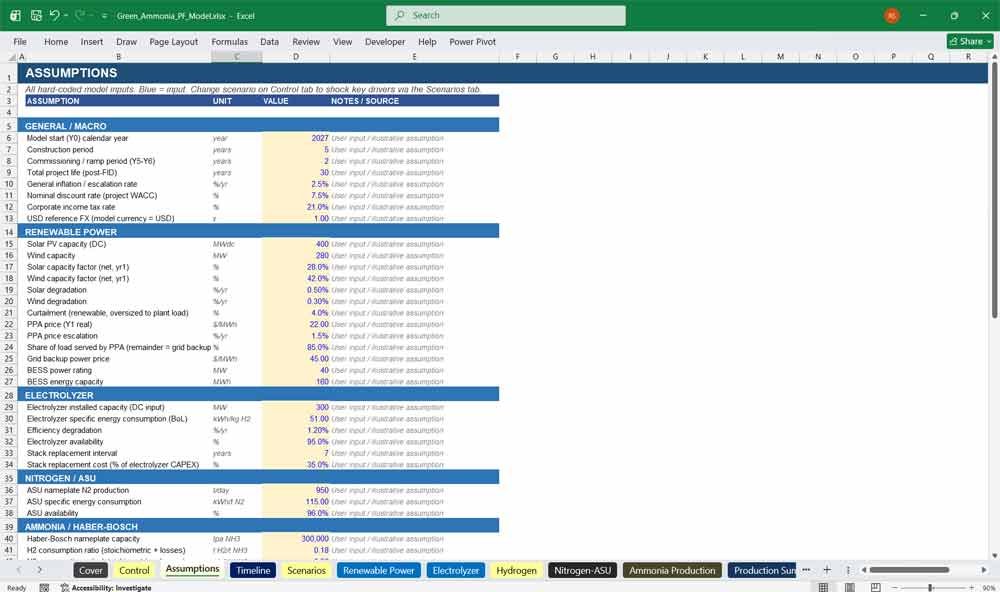
Green Ammonia Project Phasing

Timeline

The clock the whole project runs on, in months where it matters and years where it doesn’t

Timeline does two jobs at once. At the annual level, it maps out the project’s phases year by year — development, EPC award, major equipment, installation, commissioning, ramp-up, and steady-state operations — and carries the utilization ramp curve that every production tab reads from. Below that sits genuine monthly detail for the first 84 months (construction through the end of the ramp), including the S-curve spending profile that governs how capital gets drawn down and a month-by-month production ramp-up percentage. This is the tab that makes it possible to model a five-year construction period honestly instead of pretending it happens in a single annual bucket.

Genuine 84 Month detailed construction phase
S Curve Profiling

Scenarios

Base, Upside, and Downside, wired to actually move the model

Rather than a static sensitivity table, Scenarios holds seven key drivers — ammonia price, CAPEX, availability, power price, opex, interest rate, and construction delay — each with a Base, Upside, and Downside value, and an active column driven live by the Control tab’s scenario selector. Every other tab in the model references the active column, not the base case directly, so flipping one switch on Control genuinely re-flows production, revenue, financing, and returns simultaneously, rather than requiring someone to manually chase down every assumption that needs to change.

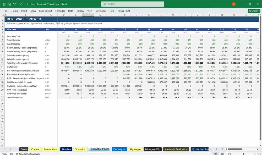
Green Hydrogen Facility Power Capacity Inputs

Renewable Power

Solar and wind generation against what the electrolyzer actually needs.

This tab models the renewable supply side on its own physical terms: solar and wind capacity degrading independently over time, capacity factors, and a curtailment allowance, netting down to the generation actually available to the plant. It then compares that supply directly against the electrolyzer’s electricity demand — pulled live from the Electrolyzer tab — splitting the result into PPA-sourced megawatt-hours, grid backup megawatt-hours, and curtailed excess, before pricing both power sources with their own escalation schedules to land on a single blended power cost. This is where the tension at the heart of green hydrogen economics — how much renewable capacity you actually need to reliably feed an electrolyzer — becomes a number instead of a hand-wave.

Solar Capacity
Wind Capacity
Solar Capacity Factor (degraded)
Wind Capacity Factor (degraded)
Electrolyzer Electricity Demand

Electrolyzer

Megawatts in, hydrogen out, with degradation and stack replacement built in properly.

The Electrolyzer tab is the mechanical heart of the hydrogen production chain: installed capacity, availability, and a ramp-up utilization curve combine into effective full-load hours and total electricity consumption, which convert into hydrogen tonnage through a specific energy consumption figure that itself degrades within each stack’s operating life. Every seven years — configurable — the stack replacement flag fires, resetting efficiency back toward beginning-of-life performance and triggering a sustaining capital cost sized as a percentage of the original electrolyzer CAPEX, so the model captures the real, lumpy nature of stack replacement rather than assuming flat performance forever.

Installed Electrolyzer Capacity (DC input)

Hydrogen

The buffer between what the electrolyzer makes and what Haber-Bosch needs.

Hydrogen sits between production and consumption, tracking storage capacity, boil-off and handling losses, and the resulting volume actually available to feed ammonia synthesis. It also reports the reverse view — how much hydrogen Haber-Bosch would need to run at its own maximum output — and the resulting surplus or shortfall, which is exactly the check that determines whether the ammonia plant is capacity-constrained by its own synthesis loop or feed-constrained by upstream hydrogen supply in any given year.

H2 Produced (Electrolyzer) t/yr
H2 Storage Capacity (buffer)

Nitrogen / ASU

The air separation side of the equation — usually the one that isn’t the bottleneck

The Nitrogen and ASU tab mirrors the electrolyzer’s logic for the air separation unit: nameplate capacity, availability, and utilization combine into maximum nitrogen output, alongside the specific energy consumption that drives the unit’s own electricity draw. Because ASU capacity is comparatively cheap to build to a comfortable margin, this tab typically isn’t where a green ammonia project gets constrained — but the model checks that explicitly on the Ammonia Production tab rather than assuming it, so an undersized ASU would actually show up as a binding constraint if someone dialed the assumptions that way.

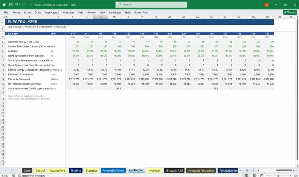
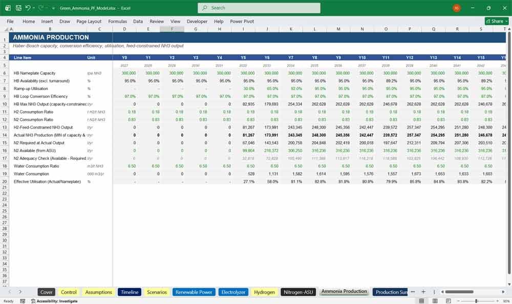
Green Ammonia Facility- Production – Capacity – Revenue

Ammonia Production

Where hydrogen, nitrogen, and Haber-Bosch capacity meet — and the real output gets decided.

This is the tab where the physical plant’s true output gets determined, and it does so honestly: Haber-Bosch nameplate capacity, availability net of scheduled turnarounds, and loop conversion efficiency define a maximum output, but actual production is the minimum of that figure and what the available hydrogen feed can support. Nitrogen requirements and water consumption are then derived from that actual output, with a running adequacy check confirming nitrogen supply never becomes the binding constraint. The result is a production number that reflects genuine plant physics rather than an assumed utilization percentage applied blindly to nameplate capacity.

HB Nameplate Capacity
Ramp-up Utilisation %
H2 Consumption Ratio / t H2/t NH3
N2 Consumption Ratio / t H2/t NH3
Water Consumption Ratio / m3/t NH3

Production Summary

Every output the plant makes, and everything it consumes to make it, in one place.

Production Summary rolls up ammonia, hydrogen, and nitrogen output alongside total electricity and water consumption, broken down by electrolyzer, ASU, and an allowance for balance-of-plant load. A specific power consumption figure — megawatt-hours per tonne of ammonia — sits at the bottom as a standing sanity check, because unit-level physics is the fastest way to catch an assumption that’s quietly gone unrealistic before it flows into revenue and cost.

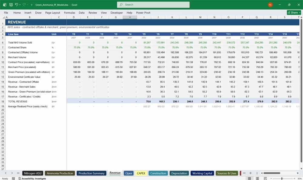
Revenue

Contracted offtake, merchant sales, green premium, and certificates — priced and escalated separately.

Revenue splits total ammonia volume into contracted offtake and merchant sales at their own escalating price tracks, then layers on a green ammonia premium and environmental certificate value across the entire volume, each with independent escalation. The four revenue streams sum to a total that’s checked against an implied average realized price per tonne — a figure worth watching closely, since it’s the single number that green ammonia economics live or die by.

Total NH3 Volume Sold
Contracted Share %
Contract Price (escalated, real+inflation) $/t

Opex

Every operating cost line, escalated on its own terms, plus the one that isn’t smooth.

Opex assembles electricity, water, catalysts and chemicals, labour, variable and fixed O&M, insurance, and SG&A, each escalating at a rate appropriate to what actually drives it — capacity-linked for fixed O&M and insurance, volume-linked for chemicals and variable O&M, inflation-linked for the rest. Electrolyzer stack replacement is smoothed into an annual accrual here rather than hitting the P&L as a single lumpy spike every seven years, which is both the more standard treatment for sustaining capital and the reason the project’s debt service coverage doesn’t crater in replacement years.

Electricity (PPA + Grid)
Catalysts / Chemicals Replacement

Capex

Every dollar of capital cost, itemized by system and phased by construction year.

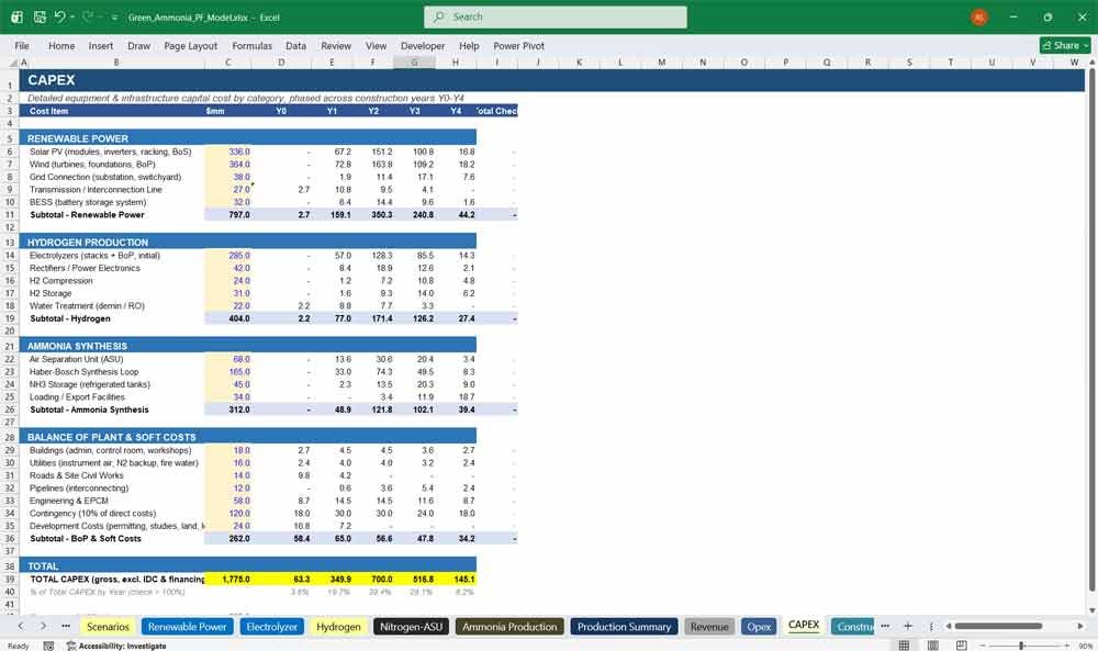
CAPEX breaks the entire capital program into four categories — renewable power, hydrogen production, ammonia synthesis, and balance of plant and soft costs — with twenty individual line items from solar PV and wind through Haber-Bosch, NH3 storage, EPCM, contingency, and development costs, each with its own construction-year phasing profile. This is the level of granularity a lender’s technical advisor would actually want to see, and it’s what the Construction tab’s monthly drawdown schedule is built on top of.

Construction

The monthly EPC drawdown, dollar for dollar, with debt and equity funding and interest capitalizing in real time.

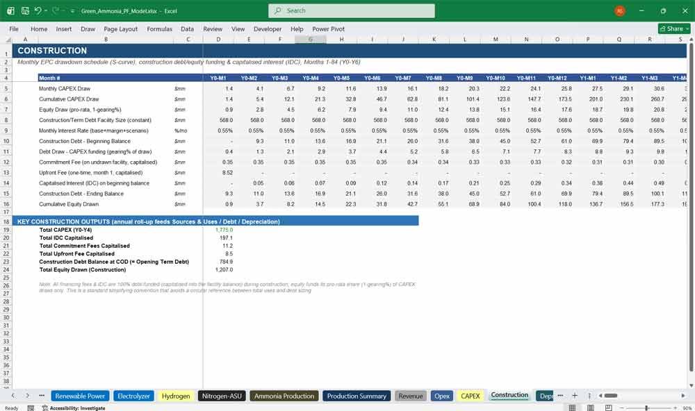
Construction is the month-by-month engine room: an S-curve spending profile spread across 84 months converts total CAPEX into a monthly draw schedule, which is funded pro-rata by equity and debt according to the target gearing ratio, with commitment fees, upfront fees, and capitalized interest accruing on the drawn debt balance every single month and compounding into the facility balance for the next. The result is a construction debt balance at completion that reflects genuine interest-during-construction cost rather than a rough estimate — and it’s meaningfully larger than the capital cost alone, which is exactly the point of modeling it this way.

Depreciation

Book and tax depreciation, tracked separately, because they should be.

Depreciation establishes a single depreciable base — total CAPEX plus capitalized interest and fees — and runs two independent straight-line schedules against it: a book life for the financial statements and a shorter tax life for the tax return, both starting at commercial operations. Keeping these separate matters because it’s precisely the gap between them that creates the deferred tax timing effects and interest-shield dynamics that make project finance debt sizing what it is.

Working Capital

Receivables, inventory, and payables, sized the way a real operating business carries them.

Working Capital applies day-based assumptions — receivable days, inventory days, payable days — against revenue and opex to build out the balances a commodity chemical producer actually carries, then converts the year-on-year change in net working capital into the cash flow impact that feeds directly into the CFADS calculation. It’s a small tab, but skipping it is one of the most common ways a project finance model quietly overstates early-year cash flow.

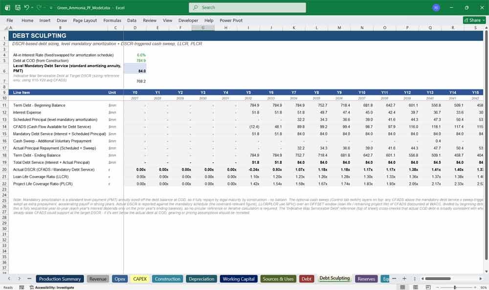
Debt Sculpting – Sizing

Where the debt sizing and repayment mechanics actually happen — level amortization plus a real cash sweep

This is the most mechanically important tab in the model. It runs the year-by-year debt balance forward from the construction-period draw, calculates interest on the beginning balance, and applies a standard level-payment amortization schedule sized off the debt balance at commercial operations — the same PMT-based mortgage math a lender would use — so the facility fully repays by legal maturity with no artificial balloon. On top of that mandatory schedule sits an optional cash sweep, active only when the Control tab switch is on, that captures cash flow available above a target coverage threshold and applies it as extra prepayment. CFADS, DSCR, LLCR, and PLCR are all calculated here too, with the entire chain built to be strictly sequential year to year — no circular references, no iterative calculation settings required, just a debt schedule that resolves the same way every time it’s opened.

Green Ammonia Facility Income Statement

Revenue to net income, the way an auditor would expect to see it.

Income Statement is the traditional P&L: revenue, cash opex, EBITDA, book depreciation, EBIT, interest expense, tax, and net income, with an EBITDA margin check running alongside it. Every line pulls from the operating, financing, and tax tabs rather than recalculating anything independently, which is what keeps this statement honest.

Cash Flow Statement

Operating, investing, and financing cash flow, reconciled down to a single closing cash balance.

Cash Flow separates operating cash flow — effectively CFADS — from investing activity, which is capital spending plus reserve account movements, and financing activity, which is debt draws and repayments alongside equity contributions and distributions. Getting the debt draw timing right here — capturing the real cash portion of construction-period draws separately from the non-cash capitalization of interest and fees into the loan balance — is what makes the cash balance actually behave the way a bank account would, rather than swinging on paper entries that never involved real money changing hands.

Balance Sheet

Assets, liabilities, and equity — and a check that confirms they actually balance, every single year

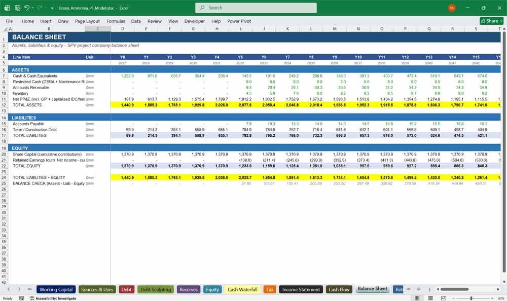
Balance Sheet builds out cash, restricted cash, receivables, inventory, and net PP&E on the asset side against payables and term debt on the liabilities side and cumulative contributed capital plus retained earnings on the equity side, with construction-period PP&E correctly including capitalized interest and fees rather than just cash-funded spend. A balance check row confirms assets equal liabilities plus equity to within a rounding tolerance in every one of the thirty-one years — not a cosmetic check, but the single most reliable way to catch a modeling error anywhere else in the workbook.

Green Ammonia Facility Returns – Valuation

The numbers that decide whether the project gets built: IRR, NPV, MOIC, and payback

Returns calculates unlevered project free cash flow and levered equity cash flow, then derives project and equity IRR, NPV at the project’s discount rate, equity multiple of invested capital, and a simple payback measure, alongside average and minimum DSCR across the stabilized operating period. This is the tab an investment committee turns to after everything else, and every figure on it is a live formula rather than a pasted-in result, so it moves the instant an assumption changes anywhere upstream.

Sensitivities

What happens if the price, the cost, or the weather doesn’t cooperate

Sensitivities lays out the live scenario summary — project IRR, equity IRR, NPV, MOIC, and DSCR under whichever scenario is currently selected on the Control tab — alongside an illustrative one-way sensitivity table showing the approximate IRR impact of shocks to ammonia price, CAPEX, power price, availability, and interest rates. The precise, fully re-solved answer to any of these questions is always available by changing the relevant input directly on the Assumptions or Scenarios tab and reading the Returns tab, since the entire model — three statements and DSCR profile included — re-flows automatically from a single changed cell.

Checks

The tab that decides whether any of the other thirty can be trusted

Checks runs ten independent integrity tests against the rest of the workbook: sources equal uses, the balance sheet ties every year, the construction S-curve sums to one hundred percent, DSCR stays above the minimum threshold through the stabilized operating period, cash never goes negative, the term debt fully amortizes by legal maturity, nitrogen supply never falls short, ammonia production never exceeds nameplate capacity, CAPEX phasing sums to the total, and debt plus equity at completion reconcile exactly to total uses — rolled up into a single master pass or fail result. A model with thirty tabs of formulas is only as trustworthy as its worst undetected error, and this tab exists to make sure there isn’t one.

Final Notes on the Green Ammonia Financial Model

This 30-Year Green Ammonia Facility Financial Model helps to focus on balancing capital expenditures with steady revenue growth from diversified distribution services. By optimizing operational costs, power efficiency, and maximizing high-margin services, the model ensures sustainable profitability and cash flow stability.

Further Reading

Hydrogen Plant Model: Download a professional Hydrogen Plant financial model. Dynamic valuation, analysis, synergies, and debt schedules.
Green Hydrogen Desalination DCF Financial Model: Create accurate financial forecasts for your Green Hydrogen Desalination. Download a powerful financial model with built-in formulas, dashboards, and easy-to-edit assumptions.